Kelly & Pruitt (2013): Summary Statistics and Replication Walkthrough

This notebook provides a guided tour of the data and methodology used to replicate Table 1 of:

Kelly, B. and Pruitt, S. (2013), “Market Expectations in the Cross-Section of Present Values.” The Journal of Finance, 68: 1721-1756.

The core insight is that a single factor extracted from the cross-section of book-to-market (BM) ratios can forecast aggregate market returns. The extraction uses a three-pass regression filter (also known as partial least squares / PLS), which is designed to handle large panels of predictors even when the time series is short.

We walk through:

1. Data Ingestion & Cleaning — How we process Fama-French portfolio data

2. Summary Statistics — Descriptive statistics for BM ratios and market returns

3. Data Sparsity — Availability of cross-sectional predictors over time

4. The Three-Pass Regression Filter — Visualizing each intermediate stage

5. Table 1 Results — Comparing our replication to the published values

import pandas as pd
import numpy as np
from IPython.display import Image, display, Markdown
from pathlib import Path

# Import our custom modules
import load_data
import regression_tools as rt
from settings import config

OUTPUT_DIR = Path(config("OUTPUT_DIR"))
START_TRAIN_DATE = config("START_TRAIN_DATE")
START_TEST_DATE = config("START_TEST_DATE")
END_TEST_DATE = config("END_TEST_DATE")

# Load all cleaned datasets
data = load_data.clean_kelly_pruitt_data(load_from_cache=True)
print(f"Loaded {len(data)} datasets: {list(data.keys())}")

Loaded 7 datasets: ['Market_Returns', '6_Portfolios_2x3_Returns', '6_Portfolios_2x3_BM', '25_Portfolios_5x5_Returns', '25_Portfolios_5x5_BM', '100_Portfolios_10x10_Returns', '100_Portfolios_10x10_BM']

1. Data Ingestion & Cleaning

We use data from Kenneth French’s data library rather than constructing portfolios directly from CRSP/Compustat. This provides pre-formed portfolios sorted on Size and Book-to-Market going back to 1926, which is critical since the paper’s training sample begins in 1930.

The raw data contains missing value indicators (-99.99, -999, etc.) which we standardize to NaN. We then construct monthly log book-to-market ratios following Vuolteenaho’s methodology:

\[\text{BM}_{i,t} = \log\left(\frac{\text{BE}_{i,Y}}{\text{ME}_{i,t}}\right)\]

where book equity (BE) is updated annually and market equity (ME) is observed monthly.

# Examine the 25 Portfolios (5x5 Size x BM) — our primary replication dataset
bm_25 = data["25_Portfolios_5x5_BM"]
print(f"25 Portfolios BM shape: {bm_25.shape}")
print(f"Date range: {bm_25.index.min().strftime('%Y-%m')} to {bm_25.index.max().strftime('%Y-%m')}")
print(f"Number of portfolios: {bm_25.shape[1]}")
print(f"\nFirst 5 rows:")
display(bm_25.head())

25 Portfolios BM shape: (1140, 25)
Date range: 1930-01 to 2024-12
Number of portfolios: 25

First 5 rows:

	SMALL LoBM	ME1 BM2	ME1 BM3	ME1 BM4	SMALL HiBM	ME2 BM1	ME2 BM2	ME2 BM3	ME2 BM4	ME2 BM5	...	ME4 BM1	ME4 BM2	ME4 BM3	ME4 BM4	ME4 BM5	BIG LoBM	ME5 BM2	ME5 BM3	ME5 BM4	BIG HiBM
Date
1930-01-01	NaN	NaN	NaN	NaN	NaN	NaN	NaN	NaN	NaN	NaN	...	NaN	NaN	NaN	NaN	NaN	NaN	NaN	NaN	NaN	NaN
1930-02-01	NaN	NaN	NaN	NaN	NaN	NaN	NaN	NaN	NaN	NaN	...	NaN	NaN	NaN	NaN	NaN	NaN	NaN	NaN	NaN	NaN
1930-03-01	NaN	NaN	NaN	NaN	NaN	NaN	NaN	NaN	NaN	NaN	...	NaN	NaN	NaN	NaN	NaN	NaN	NaN	NaN	NaN	NaN
1930-04-01	NaN	NaN	NaN	NaN	NaN	NaN	NaN	NaN	NaN	NaN	...	NaN	NaN	NaN	NaN	NaN	NaN	NaN	NaN	NaN	NaN
1930-05-01	NaN	NaN	NaN	NaN	NaN	NaN	NaN	NaN	NaN	NaN	...	NaN	NaN	NaN	NaN	NaN	NaN	NaN	NaN	NaN	NaN

5 rows × 25 columns

# Market returns — our target variable
mkt = data["Market_Returns"]
print(f"Market Returns shape: {mkt.shape}")
print(f"Date range: {mkt.index.min().strftime('%Y-%m')} to {mkt.index.max().strftime('%Y-%m')}")
print(f"Columns: {list(mkt.columns)}")
print(f"\nFirst 5 rows:")
display(mkt.head())

Market Returns shape: (1140, 4)
Date range: 1930-01 to 2024-12
Columns: ['Mkt', 'Log_Mkt', 'Mkt-RF', 'RF']

First 5 rows:

	Mkt	Log_Mkt	Mkt-RF	RF
Date
1930-01-01	5.75	0.055908	5.61	0.14
1930-02-01	2.80	0.027615	2.50	0.30
1930-03-01	7.44	0.071762	7.09	0.35
1930-04-01	-1.84	-0.018571	-2.05	0.21
1930-05-01	-1.40	-0.014099	-1.66	0.26

2. Summary Statistics

Below we compute descriptive statistics for the log BM ratios of the 25 portfolios and the log market return over the sample period used for replication (1930–2010).

# Restrict to the replication sample period
v_df = bm_25.loc[START_TRAIN_DATE:END_TEST_DATE]
y_1m = mkt['Log_Mkt'].loc[START_TRAIN_DATE:END_TEST_DATE]

print(f"Sample period: {v_df.index.min().strftime('%Y-%m')} to {v_df.index.max().strftime('%Y-%m')}")
print(f"Number of monthly observations: {len(v_df)}")
print(f"\n--- Log Book-to-Market Ratios (25 Portfolios) ---")
summary = v_df.describe().T[['mean', 'std', 'min', '25%', '50%', '75%', 'max']]
display(summary.style.format('{:.4f}'))

Sample period: 1930-01 to 2010-12
Number of monthly observations: 972

--- Log Book-to-Market Ratios (25 Portfolios) ---

	mean	std	min	25%	50%	75%	max
SMALL LoBM	-7.1225	3.1164	-11.1870	-9.5138	-8.5446	-5.1959	2.4288
ME1 BM2	-5.2121	2.4798	-9.6086	-7.5253	-5.4371	-2.9287	0.1205
ME1 BM3	-4.2593	2.2155	-8.0549	-6.1750	-4.2443	-2.8095	1.2058
ME1 BM4	-2.9968	1.9918	-6.5997	-4.7247	-2.7600	-1.6815	1.8881
SMALL HiBM	-1.4685	2.0233	-4.6608	-3.1608	-1.5776	0.0369	3.3623
ME2 BM1	-5.1693	2.6650	-8.9115	-7.6947	-5.4075	-3.2149	2.0465
ME2 BM2	-3.8530	2.1765	-7.0683	-5.9845	-3.9963	-2.1520	1.7511
ME2 BM3	-3.2305	2.0188	-6.5296	-5.2972	-2.8998	-1.7746	1.4129
ME2 BM4	-2.4647	1.9121	-5.8717	-4.0251	-2.3457	-1.1363	2.0748
ME2 BM5	-1.3422	1.6936	-4.3707	-2.8560	-1.1752	-0.0471	2.7465
ME3 BM1	-4.5319	2.2595	-8.1315	-6.7134	-4.5493	-2.7671	0.6780
ME3 BM2	-3.4057	2.0685	-6.6540	-5.4026	-3.4496	-1.7100	1.1729
ME3 BM3	-2.7606	1.8726	-6.2507	-4.5006	-2.6471	-1.2660	1.3716
ME3 BM4	-2.3256	1.8945	-5.6962	-4.1643	-2.1399	-0.9566	2.1593
ME3 BM5	-1.5689	1.4570	-4.3376	-3.0505	-1.3310	-0.5980	2.6489
ME4 BM1	-3.9582	1.9041	-7.3368	-5.5750	-3.8578	-2.2805	0.1895
ME4 BM2	-2.9957	1.8493	-6.5125	-4.6585	-2.8099	-1.6612	0.8773
ME4 BM3	-2.6628	2.0080	-6.0253	-4.4868	-2.6498	-1.0990	1.6559
ME4 BM4	-2.1654	1.9831	-5.3319	-4.3333	-1.8407	-0.4467	1.6794
ME4 BM5	-1.8780	1.3962	-4.5241	-3.1179	-1.8054	-0.8312	2.9061
BIG LoBM	-3.4723	2.0053	-7.5606	-5.1500	-3.1977	-1.6548	-0.1759
ME5 BM2	-2.9210	2.0348	-6.9424	-4.2277	-2.6352	-1.2901	1.0540
ME5 BM3	-2.4571	1.6474	-5.4731	-3.8134	-2.4652	-1.6701	2.4091
ME5 BM4	-2.3181	1.6118	-5.6255	-3.8510	-2.1239	-1.0701	2.7700
BIG HiBM	-2.8812	1.1103	-4.9414	-3.6258	-3.0644	-2.1896	1.2707

# Market return statistics
print("--- Log Market Return ---")
mkt_stats = y_1m.describe()[['mean', 'std', 'min', '25%', '50%', '75%', 'max']]
mkt_summary = pd.DataFrame(mkt_stats).T
mkt_summary.index = ['Log Market Return']
display(mkt_summary.style.format('{:.4f}'))

print(f"\nAnnualized mean return: {y_1m.mean() * 12:.4f}")
print(f"Annualized volatility:  {y_1m.std() * np.sqrt(12):.4f}")
print(f"Sharpe ratio (approx):  {(y_1m.mean() * 12) / (y_1m.std() * np.sqrt(12)):.4f}")

--- Log Market Return ---

	mean	std	min	25%	50%	75%	max
Log Market Return	0.0075	0.0545	-0.3384	-0.0185	0.0124	0.0391	0.3287

Annualized mean return: 0.0899
Annualized volatility:  0.1887
Sharpe ratio (approx):  0.4766

3. Analyzing Data Sparsity

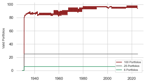
Not all portfolios have data going back to 1926. The 6-portfolio set (2×3) has near-complete coverage, but the 100-portfolio set (10×10) is sparse in early decades because many Size × BM bins lack sufficient firms. This motivates the PLS approach — it gracefully handles unbalanced panels.

# Count valid (non-NaN) portfolios at each date
bm_6 = data["6_Portfolios_2x3_BM"]
bm_100 = data["100_Portfolios_10x10_BM"]

sparsity = pd.DataFrame({
    '6 Portfolios': bm_6.count(axis=1),
    '25 Portfolios': bm_25.count(axis=1),
    '100 Portfolios': bm_100.count(axis=1)
})

print("Portfolio availability at key dates:")
key_dates = ['1930-01-01', '1950-01-01', '1970-01-01', '1990-01-01', '2010-01-01']
for d in key_dates:
    nearest = sparsity.index[sparsity.index >= pd.Timestamp(d)][0]
    row = sparsity.loc[nearest]
    print(f"  {nearest.strftime('%Y-%m')}: 6-port={row['6 Portfolios']:.0f}, "
          f"25-port={row['25 Portfolios']:.0f}, 100-port={row['100 Portfolios']:.0f}")

Portfolio availability at key dates:
  1930-01: 6-port=0, 25-port=0, 100-port=0
  1950-01: 6-port=6, 25-port=25, 100-port=87
  1970-01: 6-port=6, 25-port=25, 100-port=95
  1990-01: 6-port=6, 25-port=25, 100-port=97
  2010-01: 6-port=6, 25-port=25, 100-port=96

display(Image(filename=OUTPUT_DIR / "data_sparsity.png"))

4. The Three-Pass Regression Filter

The core methodology extracts a single predictive factor \(F_t\) from the cross-section of BM ratios. We demonstrate each stage using the 25 Portfolios with a 1-month forecast horizon (\(h=1\)).

Stage 1: Time-Series Regressions (Estimating Sensitivities)

For each portfolio \(i\), we estimate its sensitivity to future market returns via a time-series regression:

\[v_{i,t} = \phi_{i,0} + \phi_i \, y_{t+h} + e_{i,t}\]

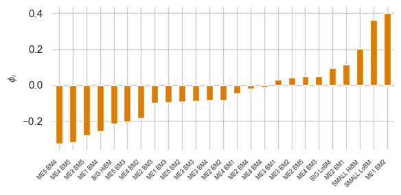
The slope coefficient \(\phi_i\) measures how much portfolio \(i\)’s BM ratio moves with future market returns. Portfolios with larger \(|\phi_i|\) carry more predictive information.

# Run Stage 1 on the full sample
y_full = mkt['Log_Mkt']
common_idx = bm_25.index.intersection(y_full.index)
v_aligned = bm_25.loc[common_idx]
y_aligned = y_full.loc[common_idx]

phi = rt.first_stage_regressions(v_aligned, y_aligned, h=1)
print(f"Estimated sensitivities for {len(phi)} portfolios:")
print(f"  Range: [{phi.min():.4f}, {phi.max():.4f}]")
print(f"  Mean:  {phi.mean():.4f}")
print(f"  Std:   {phi.std():.4f}")
print(f"\nTop 5 most sensitive portfolios:")
display(phi.sort_values(ascending=False).head().to_frame('phi'))

Estimated sensitivities for 25 portfolios:
  Range: [-0.3234, 0.3987]
  Mean:  -0.0420
  Std:   0.1867

Top 5 most sensitive portfolios:

	phi
ME1 BM2	0.398695
SMALL LoBM	0.361601
SMALL HiBM	0.202698
ME2 BM1	0.112671
BIG LoBM	0.095888

display(Image(filename=OUTPUT_DIR / "stage_1_sensitivities.png"))

Stage 2: Cross-Sectional Regressions (Extracting the Factor)

At each time \(t\), we regress the cross-section of BM ratios onto the estimated sensitivities:

\[v_{i,t} = c_t + F_t \, \phi_i + w_{i,t}\]

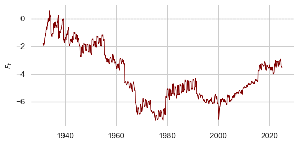
The slope \(F_t\) is our extracted latent factor — a single time series that aggregates the predictive content of all portfolios.

F_series = rt.second_stage_regressions(v_aligned, phi)
print(f"Extracted factor F_t: {len(F_series)} observations")
print(f"  Date range: {F_series.index.min().strftime('%Y-%m')} to {F_series.index.max().strftime('%Y-%m')}")
print(f"  Mean:  {F_series.mean():.4f}")
print(f"  Std:   {F_series.std():.4f}")
print(f"  Correlation with log market return: {F_series.corr(y_aligned.reindex(F_series.index)):.4f}")

Extracted factor F_t: 1122 observations
  Date range: 1931-07 to 2024-12
  Mean:  -4.0974
  Std:   1.9494
  Correlation with log market return: 0.0241

display(Image(filename=OUTPUT_DIR / "stage_2_factor.png"))

Stage 3: Predictive Regression

Finally, we regress future market returns on the lagged factor:

\[y_{t+h} = \beta_0 + \beta \, F_t + u_{t+h}\]

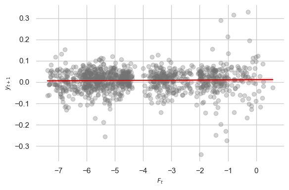
If \(F_t\) captures genuine predictive information, \(\beta\) should be statistically significant and the \(R^2\) should be meaningfully positive.

model = rt.third_stage_regression(F_series, y_aligned, h=1)
print("Stage 3 Predictive Regression Results:")
print(f"  Intercept (beta_0): {model.params.iloc[0]:.6f}")
print(f"  Slope (beta):       {model.params.iloc[1]:.6f}")
print(f"  In-sample R²:       {model.rsquared:.4f} ({model.rsquared * 100:.2f}%)")
print(f"  t-stat (slope):     {model.tvalues.iloc[1]:.4f}")
print(f"  p-value (slope):    {model.pvalues.iloc[1]:.4f}")
print(f"  N observations:     {int(model.nobs)}")

Stage 3 Predictive Regression Results:
  Intercept (beta_0): 0.011377
  Slope (beta):       0.000712
  In-sample R²:       0.0007 (0.07%)
  t-stat (slope):     0.8927
  p-value (slope):    0.3722
  N observations:     1121

display(Image(filename=OUTPUT_DIR / "stage_3_predictive.png"))

5. Table 1 Replication Results

Table 1 reports in-sample (IS) and out-of-sample (OOS) predictive \(R^2\) values across three portfolio granularities (6, 25, 100) and two forecast horizons (1-month, 1-year). The out-of-sample evaluation uses an expanding window — at each test date, the model is re-estimated using only data available up to that point.

We compare our replication against the published values:

# Load pre-computed Table 1 results (from replication.py pipeline)
try:
    df_original = pd.read_csv(OUTPUT_DIR / "table_1_results_original.csv", index_col=0)
    
    # Published values from the paper
    paper_values = pd.DataFrame({
        "1-Year IS": {"6 Portfolios": 7.72, "25 Portfolios": 13.50, "100 Portfolios": 18.05},
        "1-Year OOS": {"6 Portfolios": 5.81, "25 Portfolios": 3.49, "100 Portfolios": 13.07},
        "1-Month IS": {"6 Portfolios": 0.60, "25 Portfolios": 1.12, "100 Portfolios": 2.38},
        "1-Month OOS": {"6 Portfolios": 0.65, "25 Portfolios": 0.77, "100 Portfolios": 0.93},
    })
    paper_values.index.name = "Portfolio Set"
    
    print("=" * 70)
    print("PUBLISHED VALUES (Kelly & Pruitt 2013, Table 1)")
    print("=" * 70)
    display(paper_values.style.format('{:.2f}'))
    
    print("\n" + "=" * 70)
    print("OUR REPLICATION (Train: 1930-1980, Test: 1980-2010)")
    print("=" * 70)
    display(df_original.style.format('{:.2f}'))
    
    # Compute differences
    diff = df_original - paper_values
    print("\n" + "=" * 70)
    print("DIFFERENCE (Replication - Published)")
    print("=" * 70)
    display(diff.style.format('{:+.2f}'))
    
except FileNotFoundError:
    print("Table 1 results not yet computed. Run 'doit run_replication' first.")
    print("(The out-of-sample expanding window computation takes ~20 minutes.)")

======================================================================
PUBLISHED VALUES (Kelly & Pruitt 2013, Table 1)
======================================================================

	1-Year IS	1-Year OOS	1-Month IS	1-Month OOS
Portfolio Set
6 Portfolios	7.72	5.81	0.60	0.65
25 Portfolios	13.50	3.49	1.12	0.77
100 Portfolios	18.05	13.07	2.38	0.93

======================================================================
OUR REPLICATION (Train: 1930-1980, Test: 1980-2010)
======================================================================

	1-Year IS	1-Year OOS	1-Month IS	1-Month OOS
Portfolio Set
6 Portfolios	1.08	-6.66	0.15	-0.32
25 Portfolios	0.92	-6.12	0.08	-1.13
100 Portfolios	2.14	-6.81	0.31	-1.09

======================================================================
DIFFERENCE (Replication - Published)
======================================================================

	1-Year IS	1-Year OOS	1-Month IS	1-Month OOS
Portfolio Set
6 Portfolios	-6.64	-12.47	-0.45	-0.97
25 Portfolios	-12.58	-9.61	-1.04	-1.90
100 Portfolios	-15.91	-19.88	-2.07	-2.02

# Modern period extension
try:
    df_modern = pd.read_csv(OUTPUT_DIR / "table_1_results_modern.csv", index_col=0)
    print("=" * 70)
    print("REPRODUCTION WITH NEW DATA (Train: 1930-2010, Test: 2011-2024)")
    print("=" * 70)
    display(df_modern.style.format('{:.2f}'))
except FileNotFoundError:
    print("Modern period results not yet computed.")

======================================================================
REPRODUCTION WITH NEW DATA (Train: 1930-2010, Test: 2011-2024)
======================================================================

	1-Year IS	1-Year OOS	1-Month IS	1-Month OOS
Portfolio Set
6 Portfolios	0.66	-1.12	0.07	-0.57
25 Portfolios	0.92	3.50	0.07	-0.12
100 Portfolios	1.76	-1.27	0.21	-0.46